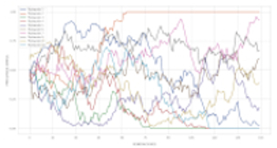
In the simulator, the population size N corresponds to the effective population size N_e as long as there is no mutation or selection, since mating is random and by default self-fertilization is allowed. Random fluctuations in the allele frequency q will manifest as an increase in the variance of the allele frequency σ²_q between different subpopulations or replicates. For the same number of populations and generations we will see that the variance increases more rapidly if N_e is low. For example, with 20 populations we can see in Figure 1 the comparison between the case N_e=10 and N_e=1000 after 100 generations of evolution.

A    N_e = 10

B     N_e = 1000

The mean frequency value in Figure 1 after 100 generations is in both cases around 0.5 but the variance with N_e=10 is close to the maximum (0.25 ) while with N_e=1000 it is 0.01. The drift generates dispersion of the frequencies in the different lines. What we observe in Figure 1 is that this dispersion occurs faster when N_e is smaller, which is visually appreciated by the separation between the different lines. This is consistent with what is predicted by the formulas for F_t and σ²_q of Figure 2.

The drift effect is mediated by the quantity 2N_e which, in turn, affects the variance σ² _q of the frequency between lines. In the absence of other forces, the expected allele frequency does not change but the between-line variance increases, and after a sufficient number of generations it will reach its maximum value p₀q₀, which occurs when all populations have their frequency at 0 or 1, that is, all lines are fixed (F_t=1). If N_e is small, this value will be reached more quickly, as we can see in Figure 1. On the contrary, if N _e is large, there is less drift, and the variance increases more slowly. To appreciate the effect of the drift on the variance of the allele frequency we can use the simulator, for example, setting the number of populations to 20, playing with different population sizes and leaving the rest of the default parameters. 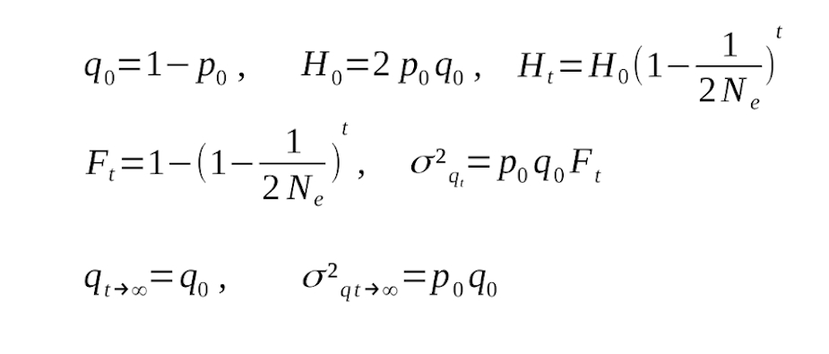Figure 2 shows the mathematical relationship between drift and genetic variability. Use the formulas that appear there to solve the following exercises.

 

In the drift model, the variance between lines is initially 0 because the initial frequency q₀ is the same for all populations. In several experiments during 3 generations the variance increased by more than 20%. The variance in the third generation was 0.21. If the initial allele frequency was 0.5 and there is no mutation or selection, what was the effective populaton size? Check it by simulation.

 

Initially q₀=0.5 and at t=3, σ²_q3=0.21 then 0.21=0.25×F₃ and solving, F₃=0.84. The relationship with the effective population size is 0.84=1-(1-1/(2N_e))³. Therefore (1-1/(2N_e))³=0.16. Taking the cube root of both sides of the equality and solving for N_e we get 1-1/(2N_e )=0.543 => 0.457=1/(2N_e) => N_e≈1.

100 populations with initial frequency q₀=0.5 were simulated. After 5 generations the variance of q was approximately 0.1. There is no mutation or selection. Would you say that the effective population size is around 5 or 50? Justify your answer and check it by means of a simulation.

 

Remember that the lower the effective population size, the faster the increase in variance. We know that σ²_q5=p₀q₀F₅. Since p₀=q₀=0.5 and σ²_q5≈0.1 we have 0.1= 0.25×F₅ and solving, F₅=0.4.
If it were N_e=5 then F₅=1-(1-1/(2N_e))⁵=1-(1-1/(10))⁵=0.41.
If it were N_e=50 then F₅=1-(1-1/(2N_e))⁵=1-(1-1/(100))⁵=0.05.
With which it seems that the effective size is around 5 and not 50. Which we can easily check by performing a simulation with parameters n=100, q₀=0.5, t=5 without mutation or selection and testing first N_e=5 and then N_e=50. And checking in each case the value of the variance obtained (we expect it to be approximately 0.1).

What will be the minimum number of generations necessary so that in a set of populations of size 5, the variance between lines obtained is half the maximum variance? HINT: Remember that the maximum variance is p₀q₀.

 

If N_e=5 then F_t=1-(1-1/10)^t=1-0.9^t. Since σ²_qt=p₀q₀F_t we have that p₀q₀/2=p₀q₀F_t and therefore F_t=0.5=1-0.9^t=>0.9^t=0.5. Taking logarithms to both sides, t=log(0.5)/log(0.9)=6.6≈7 will be the minimum number of generations needed.